Difficulty Estimating a Multivariate Normal Outcome

[NathanielF]

Hi All,

I’m trying to develop a better understanding of the amortized bayesian inference procedures and maybe compare them with vanilla bayesian modelling and/or VAE methods.

So i thought i’d try and do a parameter recovery exercise on a multivariate normal outcome. I have code working that i think is doing what it should do, but the estimation is super slow and for this “simple” example i feel i must have gotten something wrong in the set up. Could you advise if i’ve got the procedure right?

Generate Data

import pandas as pd
import numpy as np
import bayesflow as bf

# Standard deviations
stds = np.array([0.939, 1.017, 0.937, 0.562, 0.760, 0.524, 
                 0.585, 0.609, 0.731, 0.711, 1.124, 1.001])

n = len(stds)

# Lower triangular correlation values as a flat list
corr_values = [
    1.000,
    .668, 1.000,
    .635, .599, 1.000,
    .263, .261, .164, 1.000,
    .290, .315, .247, .486, 1.000,
    .207, .245, .231, .251, .449, 1.000,
   -.206, -.182, -.195, -.309, -.266, -.142, 1.000,
   -.280, -.241, -.238, -.344, -.305, -.230,  .753, 1.000,
   -.258, -.244, -.185, -.255, -.255, -.215,  .554,  .587, 1.000,
    .080,  .096,  .094, -.017,  .151,  .141, -.074, -.111,  .016, 1.000,
    .061,  .028, -.035, -.058, -.051, -.003, -.040, -.040, -.018,  .284, 1.000,
    .113,  .174,  .059,  .063,  .138,  .044, -.119, -.073, -.084,  .563,  .379, 1.000
]

# Fill correlation matrix
corr_matrix = np.zeros((n, n))
idx = 0
for i in range(n):
    for j in range(i+1):
        corr_matrix[i, j] = corr_values[idx]
        corr_matrix[j, i] = corr_values[idx]
        idx += 1

# Covariance matrix: Sigma = D * R * D
cov_matrix = np.outer(stds, stds) * corr_matrix
columns=["JW1","JW2","JW3", "UF1","UF2","FOR", "DA1","DA2","DA3", "EBA","ST","MI"]
corr_df = pd.DataFrame(corr_matrix, columns=columns)

cov_df = pd.DataFrame(cov_matrix, columns=columns)
cov_df

def make_sample(cov_matrix, size, columns):
    sample_df = pd.DataFrame(np.random.multivariate_normal([0]*12, cov_matrix, size=size), columns=columns)
    return sample_df

sample_df = make_sample(cov_matrix, 263, columns)
sample_df.head()

Which gives us a data set like:

What i’m interested in doing is estimating the covariance parameters which generated that sample. So i tried following the docs and set up my simulator and adapter etc so that i can do diagnostic tests and then ultimately calibrate the model against the observed sample data.

def random_corr(dim):
    A = np.random.randn(dim, dim)
    Q, _ = np.linalg.qr(A)   # orthogonal matrix
    R = Q @ Q.T              # PD correlation-like
    D = np.diag(1 / np.sqrt(np.diag(R)))
    return D @ R @ D

def random_cov_lkj(dim):
    R = random_corr(dim)
    stds = np.exp(np.random.randn(dim))  # log-normal stds
    D = np.diag(stds)
    return D @ R @ D

def likelihood(mu, sigma):
    N = sample_df.shape[0]
    dim = sample_df.shape[1]
    Sigma = sigma.reshape(dim, dim)
    return {"y": np.random.multivariate_normal(mu, Sigma, size=N)}

def prior():
    dim = sample_df_missing.shape[1]
    mus = np.random.normal(0, 1, size=dim)
    sigma = random_cov_lkj(dim)
    return {"mu": mus, "sigma": sigma.ravel()}

simulator = bf.make_simulator([prior, likelihood])
sims=simulator.sample(1)

adapter = (
    bf.Adapter()
    .as_set(["y"])
    .convert_dtype("float64", "float32")
    .concatenate(["mu", "sigma"], into="inference_variables")
    .concatenate(['y'], into='summary_variables')
)


summary_network = bf.networks.SetTransformer(summary_dim=10)

workflow = bf.BasicWorkflow(
    simulator=simulator,
    adapter=adapter,
    summary_network=summary_network,
    inference_network = bf.networks.CouplingFlow(),
    inference_variables="y",
    inference_conditions=["mu", "sigma"],
    initial_learning_rate=1e-3,
    standardize=None
)

training_data = workflow.simulate(1000)
validation_data = workflow.simulate(300)
## Runs but slowly
history = workflow.fit_offline(data=training_data, epochs=10, validation_data=validation_data);
bf.diagnostics.loss(history);

This code runs but does so quite slowly. Have i parameterised this poorly? I tried to recreate sampling of the covariance rather than say install pymc and sample from the LKJ prior… but i guess i could have done so poorly or inefficiently.

Ultimately i’m more interested in ensuring that the calibratio step works to estimate the posterior

post = workflow.sample(num_samples=200, conditions={'y': sample_df.values[None, :]})

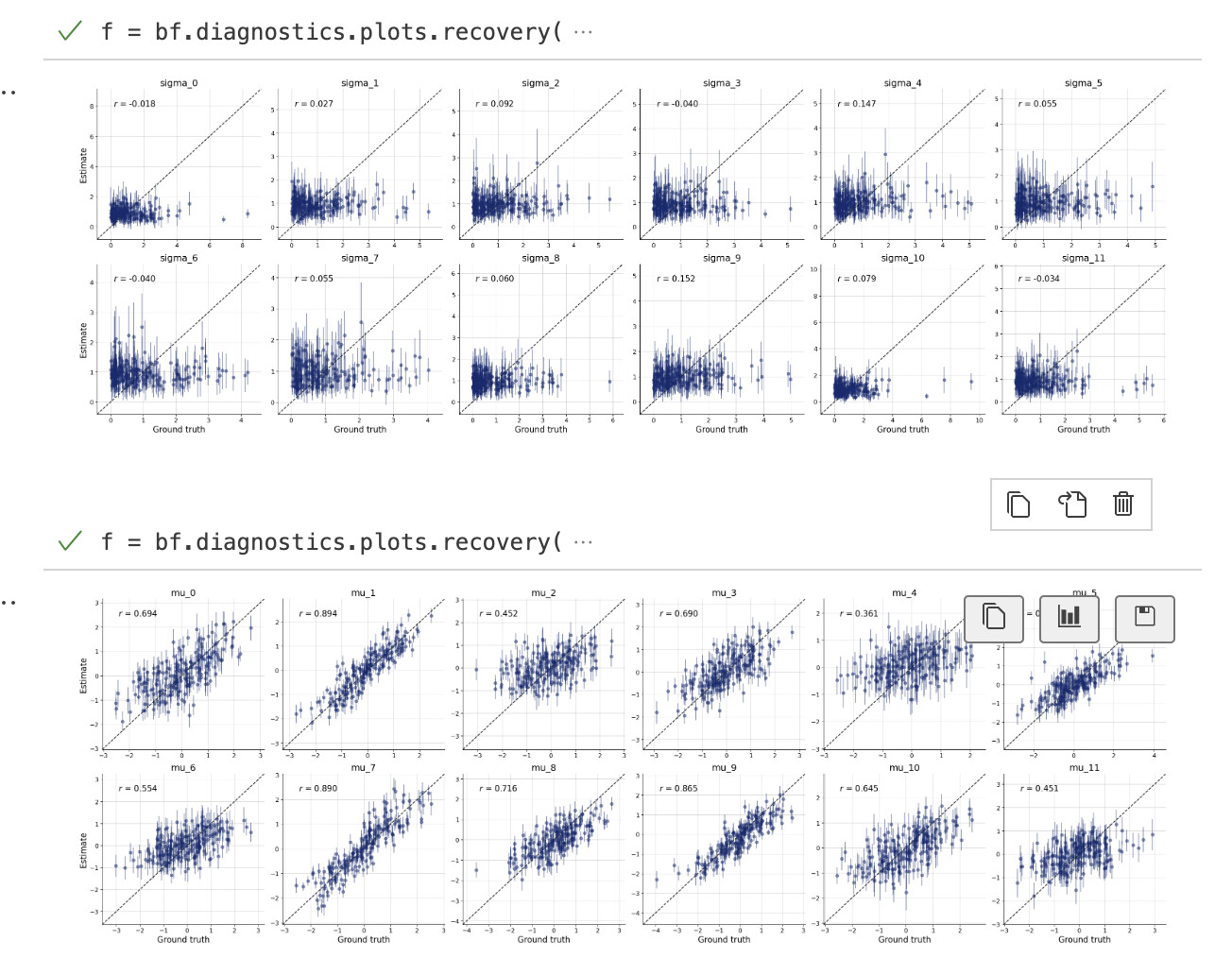
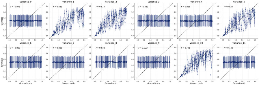
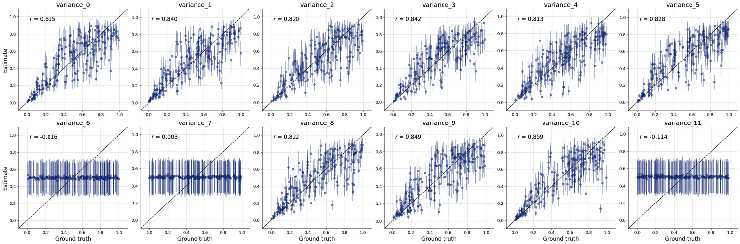
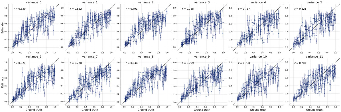
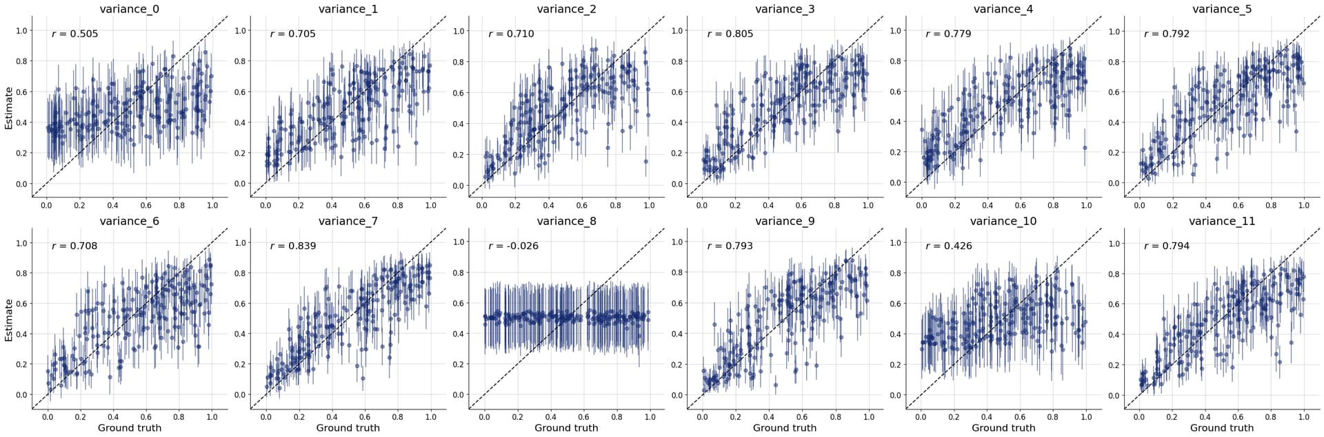
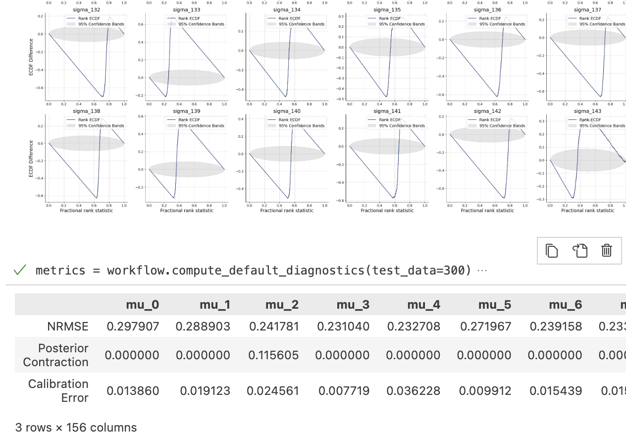
But i’m not sure if i’ve set up the whole workflow properly so i don’t really trust the posterior estimates. The diagnostic checks on the online process seem to suggest that it’s poorly specified too

Would you be able to advise if i’m on the right track? Or where i should go to ask for pointers on this use case? Thanks for your hard work and this cool looking package!

[valentin]

Hi Nathaniel,
welcome to the forum. I just ran your code, I’ll just write down my thoughts/ideas, let me know if you have questions or I have missed something.

Data Generation

Estimating covariance matrices is quite tricky for a larger number of variables, so I would consider this already a quite challenging setting. Also, as the accuracy of neural network is limited, it can be hard to fulfill the constraints on the matrix (symmetric and positive semi-definite) without enforcing them manually. The usual way to go would to estimate the parameters of a decomposition (e.g., Cholesky), which ensures that those constraints are fulfilled by design.

I noticed the simulator produces off-diagonal values that are basically zero, and have very little variation:

>>> sims = simulator.sample(100)
>>> sims['sigma'].mean(0)
array([ 7.87386082e+00, -8.68711289e-17,  1.20736712e-16,  5.29001955e-18,
       -2.32990176e-17, -9.57408673e-17, -9.46165193e-17, -5.30097856e-18,
       -3.82449668e-17, ...])
>>> sims['sigma'].std(0)
array([2.06161843e+01, 1.35038634e-15, 9.65351036e-16, 7.51036488e-16,
       8.36689008e-16, 9.73089520e-16, 9.53742296e-16, 4.74288416e-16,
       8.72537982e-16, ...])

For your tests, I would suggest you use a prior that produces non-zero covariances, like the LKJ prior you suggested. Or you exclude the covariances for now, and only estimate the variances. This would then be an easy problem.

Estimation

The posterior contraction of 0 on the mu parameters suggests that no successful training has happened yet, as we would expect good estimation of the means for the given number of samples from the distribution.

Speed

The slow estimation is mainly due to using a transformer (SetTransformer), which is slow unless you have a GPU available. Changing this to a DeepSet increases the speed by a factor of ~6 (to 125ms/step on my Laptop using TensorFlow, after the initial compilation is finished). In addition, the number of parameters you want to estimate is not super low, which also increases training time.

Standardization

If you have variables that are not in the standard range of ±10, enabling standardization usually makes sense. Transformers are especially sensitive to this in my experience. So I would suggest passing standardize="summary_variables" to the workflow.

Summary dimensions

As you want to estimate twelve independent means and the covariance matrix, you will need more summary dimensions so that all information can be passed to the inference network. The exact number depends on the setting, one rule of thumb is the number of minimal sufficient statistics times two. Here I think this would be 78 for the covariance matrix and 12 for the means, so 90*2, but for testing I would start with something lower, e.g. 64, and then see how the results change when you in/decrease the number.

---

So I’d suggest:

• work incrementally: first simulate only a diagonal covariance matrix, and estimate the variances
• if this works (if it doesn’t, please reach out), you can move to full covariance matrices
• for this, find a way to sample from a diverse prior, e.g. LKJ, and a good parameterization, e.g. Cholesky.
• Then try to estimate the independent parameters, so not a full M\times M matrix, but the M\cdot (M+1)/2 independent parameters that go into the parameterization.

[NathanielF]

Thanks. I’ll experiment a bit!

[NathanielF]

Ok, i think i made some progress.

New workflow is here:

N = len(sample_df) 

def lkj_cholesky(d, eta=1.0, independent=True):
    L = np.zeros((d, d))

    # First diagonal is 1
    L[0, 0] = 1.0

    for k in range(1, d):
        # Sample the "radius" (diagonal element) using Beta distribution
        alpha = eta + (d - k - 1) / 2.0
        beta_sample = np.random.beta(alpha, alpha)
        L[k, k] = np.sqrt(beta_sample)

        # Sample the off-diagonal entries
        z = np.random.normal(size=k)
        z = z / np.linalg.norm(z) * np.sqrt(1 - L[k, k]**2)
        L[k, :k] = z

    # Build correlation matrix
    corr = L @ L.T
    sds = np.random.exponential(1, size=12)

    # Build covariance matrix
    D = np.diag(sds)
    cov = D @ corr @ D
    L = np.linalg.cholesky(cov)
    if independent:
        return D
    else:
        return L

def prior(eta=1.0, sd_scale=1.0, independent=True):
    dim = sample_df.shape[1]
    mus = np.random.normal(0, 1, size=dim)
    L = lkj_cholesky(12)
    if independent:
        ## stores params as vector
        params = np.diag(L)
    else: 
        params = L[np.tril_indices_from(L)]
    return {"mu": mus, "sigma": params}


def likelihood(mu, sigma):
    d = len(mu)
    if sigma.ndim == 1:
        ## reconstructs matrix
        Sigma = np.diag(sigma)
    else:
        L = np.zeros((d, d))
        L[np.tril_indices(d)] = sigma
        Sigma = L @ L.T
    return {"y": np.random.multivariate_normal(mu, Sigma, size=N)}


simulator = bf.make_simulator([prior, likelihood])

adapter = (
    bf.Adapter()
    .as_set(["y"])
    .convert_dtype("float64", "float32")
    .concatenate(["mu", "sigma"], into="inference_variables")
    .concatenate(['y'], into='summary_variables')
)


summary_network = bf.networks.DeepSet(summary_dim=24, 
    hidden_units=[128, 128],
    dropout_rate=0.3)

workflow = bf.BasicWorkflow(
    simulator=simulator,
    adapter=adapter,
    summary_network=summary_network,
    inference_network = bf.networks.CouplingFlow(),
    inference_variables="y",
    inference_conditions=["mu", "sigma"],
    initial_learning_rate=1e-3,
    standardize="summary_variables"
)


training_data = workflow.simulate(5000)
validation_data = workflow.simulate(300)

history = workflow.fit_offline(data=training_data, epochs=20, validation_data=validation_data, batch_size=128);

# Set the number of posterior draws you want to get
num_samples = 1000

# Simulate validation data (unseen during training)
val_sims = simulator.sample(200)

# Obtain num_samples samples of the parameter posterior for every validation dataset
post_draws = workflow.sample(conditions=val_sims, num_samples=num_samples)


f = bf.diagnostics.plots.recovery(
    estimates=post_draws, 
    targets=val_sims,
    variable_keys=['sigma']
)

This allows for the independent or diagonal covariance and the LKJ specification. I’m focused currently on the independent as you suggested. But it’s worth noting the LKJ specification also seems to sample… (albeit slowly and poorly). We re-construct a matrix in the likelihood.

Loss trajectory seems ok,However the recovery plots aren’t great:

And it takes roughly 493ms a step with pytorch. It’s much quicker for me to fit this model with NUTS and MCMC…

[valentin]

Thanks for sharing. It seems that the summary networks (both SetTransformer and DeepSet) fail to learn the relevant summary statistics required to estimate the variances. I further reduced the code to a minimal example that I would have expected to work, but it doesn’t.

import keras
import bayesflow as bf
import numpy as np

D = 12
N = 10
rng = np.random.default_rng(2025)

def prior():
    variance = rng.uniform(size=D)
    return {"variance": variance}


def likelihood(variance):
    y = rng.normal(loc=np.zeros_like(variance), scale=np.sqrt(variance), size=(N, D))
    return {"y": y}

simulator = bf.make_simulator([prior, likelihood])

validation_data = simulator.sample(100)
print("shapes", keras.tree.map_structure(keras.ops.shape, validation_data))

summary_network = bf.networks.SetTransformer(summary_dim=2*D)

workflow = bf.BasicWorkflow(
    simulator=simulator,
    summary_network=summary_network,
    summary_variables="y",
    inference_variables=["variance"],
    initial_learning_rate=1e-3,
    standardize="all",
)

workflow.fit_online(num_batches_per_epoch=1000, epochs=10, validation_data=validation_data, batch_size=32);

test_data = simulator.sample(200)

workflow.plot_default_diagnostics(test_data);

This produces the following result. While it learns the relevant summary statistics for some dimensions, it fails to do so for the others. Note that they are all interchangeable, so which one will be learned is random.

Using a SetTransformer instead of the DeepSet shows the same problem, but to a somewhat lesser degree:

I’m not sure if I missed anything, tagging @KLDivergence, @paul.buerkner, @elseml if they have any ideas or insights to share on how one would approach this.

[paul.buerkner]

I agree it should work. What happens (1) if we enforce the lower boundary of zero for variance via adapter.constrain? (2) If we replace the set networks with a basic MLP summary?

[NathanielF]

Thanks for helping folks. I can probably try and constrain the lower bound this evening. Not 100% sure what you mean for (2) @paul.buerkner , but happy to explore the networks API if that’s where this sits.

[valentin]

Thanks @paul.buerkner. (1) Does not change anything. (2) is very similar to not using a summary network at all, and this resolves the issue/changes the pattern. This indicates that the problem is indeed with the summary networks, and they pose some sort of “information bottleneck” where the information on some variables is lost. I imagine that this might be reduced by (heavily) increasing the number of summary dimensions. I’ll try that out, but it might not be a very reliable and somewhat costly way to go.

Below is the code for this setting.

import keras
import bayesflow as bf

D = 12
N = 10
rng = np.random.default_rng(2025)


def prior():
    variance = rng.uniform(size=D)
    return {"variance": variance}


def likelihood(variance):
    y = rng.normal(loc=np.zeros_like(variance), scale=np.sqrt(variance), size=(N, D))
    # flatten data for use without summary network
    return {"y": y.reshape(-1)}

simulator = bf.make_simulator([prior, likelihood])

validation_data = simulator.sample(100)
keras.tree.map_structure(keras.ops.shape, validation_data)

workflow = bf.BasicWorkflow(
    simulator=simulator,
    inference_variables="variance",
    inference_conditions="y",
    initial_learning_rate=1e-3,
    standardize="all",
)

workflow.fit_online(num_batches_per_epoch=1000, epochs=10, validation_data=validation_data, batch_size=32);

test_data = simulator.sample(200)

workflow.plot_default_diagnostics(test_data);

[valentin]

Increasing the number of summary dimensions to 10*D does not change the behavior qualitatively. @LarsKue Do you have an idea what is going on under the hood that might cause this behavior? And is this something we can improve somehow?

[paul.buerkner]

This is strange, but something I have seen also in other applications. @kucharssim or @Daniel we had this somewhere else too, right?

[LarsKue]

Could be a number of things related to training, but what stands out to me is the small set size of just 10 samples, which could lead to an uninformative summary embedding, especially because all of the distributions have the same mean.

[elseml]

I agree with @valentin’s intuition, exchanging the summary network in the minimal example with a basic MLP summary net (retaining summary_dim=2*D) further improves the pattern of ignoring single target variables compared to a SetTransformer, but does not fully eliminate it:

[paul.buerkner]

Still, N = 10 should be enough to identify a variance reasonably. So our summary networks should be able to pick that up.

[valentin]

Yes, the behavior is the same for N=263, so I think this is not related to the set size in this example. Also, it learns the correct summary statistics for some, but not all variables, even though the available information for each variable is identical.

[paul.buerkner]

Could this be an issue with intialization? Our inference networks have pretty reasonable initilization, but I don’t know if this is true for our summary networks.

[paul.buerkner]

How are we currently initializing our summary networks? Specifically our set networks

[elseml]

I don’t think that the patterns are caused by initialization since we are using rather standard initialization. I tested exchanging "lecun_normal" with "he_normal" (which arguably fits the GELU activation better) in the SetTransformer, but it has little effect. The patterns also don’t seem to be an artifact from insufficient training that eventually fades, since doubling the number of epochs has little effect for both DeepSet and SetTransformer summary nets. The issue thus seems to be some kind of inherent mismatch of the inductive bias imposed by the set network architectures for this kind of problem.

[valentin]

I have an idea, but I’m not sure how sensible it is. I believe that “switching” a summary variable to be informative about a different parameter has a high cost, as the inference network is already using the variable and discourages it from changing to something completely different.
This would mean that after the initial phase, each summary dimension belongs to one parameter. If the initial assignment is happening randomly based on the initializiation and is independent (which it generally will not be), we can calculate the number of parameters that are not assigned any summary dimension (and therefore only learning the prior) using the following simulation:

import numpy as np
import matplotlib.pyplot as plt

summary_dim = 2 * D
counts = np.random.multinomial(summary_dim, (1/D,) * D, size=100000)
num_zeros = np.sum(counts == 0, axis=1)
plt.hist(num_zeros, bins=np.arange(np.max(num_zeros) + 1) - 0.5, density=True)
plt.xlabel("Number of parameters without assigned summary variable");

For D=12, this leads to the following histogram:

Correlation in the assignment of the summary variables to the parameters would increase the number, anti-correlation (which would be desired) would move it towards zero.

Do you think this might make sense? If so, I think it would not be so hard to test empirically…

[paul.buerkner]

I do think that makes a lot of sense. Essentially, we get stuck in local minima of the of loss landscape from which we cannot recover. The question is essentially how to fix it.

[paul.buerkner]

Could it be helpful to enforce independence of summary statistics? For example our MMD loss in summary space enforces independence even if it was build for a difference purpose (OOD detection).